Linear Regression

Alphabate in the upper case is a matrix and in the lower case is a vector.

Introduction

Assume we have some \(n\) training data points \({(x_i, y_i)}_{i = 1}^{n}\) that comes from an unknown/known distribution \(\mathcal{P}_{xy}\). Where, the \(x_i \in \mathcal{X} \in \mathbb{R}^d\) comes from the input distribution \(\mathcal{P}_{x}\) and \(y_i \in \mathcal{Y} \in \mathbb{R}\) comes from a conditioned distribution \(\mathcal{P}_{y/x}\). Now, we have a new data point \(x_{n+1}\) and we need to estimate the output for that point. We can think of an example that a hospital has some patients data. \(x_i\) consists of some risk factors such as age, blood pressure, height, body weight, etc., for a patient and \(y_i\) is a measure of kidney function(e.g., eGFR) for the same patient. Using the previous \(n\) data points, our goal is to estimate the output of the new data point \(x_{n+1}\).

We can design an algorithm \(A \in \mathcal{A}\) that takes the \(n\) data points as an input and return a learned function \(f \in \mathcal{F}\) such that \(f: \mathcal{X} \rightarrow \mathcal{Y}\). Now, if we know the learned \(f\), we can estimate the new output for the \(x_{n+1}\). There are different ways to learn the \(f\) function. We will discuss some of them in this sections with python codes. We name linear regression because the predicted target value \(\hat{y}\) is expected to be a linear combination of the features of \(x\). In mathematical notation, we can write \(\hat{y}\) as follows:

\[\hat{y}(\theta, x) = \theta^{1}*x^1 + \theta^{2} * x^2 +...+ \theta^{d} * x^{d} + b\]

Where, \(\theta = [\theta^1, \theta^2, ...., \theta^d]\) is the parameters and \(b\) is the bias term. We can include the bias term within \(\theta\) such that \(\theta = [\theta^0, \theta^1, \theta^2, ...., \theta^d]\). We can calculate the error/loss term as \((\hat{y}_i - y_i)\) for the \(x_i\) data point. Our goal is to update the \(\theta\) parameters in such a way that the error term gets minimized for the future data points such as \(x_{n+1}\).

Ordinary Least Squares

Here, we try to solve a problem of the form as follows:

\[min_{\theta} ||X\theta - Y||_2^2\]

In the above equation \(\hat{y} = x \theta\) for a data point and \(\hat{Y} = X \theta\) for all \(n\) data points. Where \(\theta \in \mathbb{R}^{d+1}\). The \((+1)\) comes due to including the bias term within \(\theta\). For a new data point \(x_{n+1}\), we can estimate \(\hat{Y}_{n+1}\) as \(x_{n+1} \theta\), but we do not know the \(\theta\) parameter. One way we can assume \(\theta\) as random variables, but for a new point \(x_{n+1}\), we may have high error/loss \((y_{n+1} - \hat{y}_{n+1})\) assuming that we know \(y_{n+1}\). There are two ways to solve the above problem to get minimum error in the future data points. One is the exact solution and another one is the approximate solution.

Exact Solution

The loss for the \(n\) data points is as follows:

\[L = ||X\theta - Y||_2^2\]

We need to find \(\theta\) that minimizes the \(L\) term.

\[ \begin{align}\begin{aligned}L &= (X \theta - Y)^T(X \theta - Y)\\ &=(\theta^T X^T - Y^T)(X \theta - Y)\\ &= \theta^T X^T X \theta - \theta^T X^T Y - Y^T X \theta + Y^T Y\\ &= \theta^T X^T X \theta - 2 Y^T X \theta + Y^T Y\\\frac{\partial L}{\partial \theta} &= 2 \theta^T X^T X - 2 Y^T X\\ &= 0\\\theta^T X^T X &= Y^T X\\X^T X \theta &= X^T Y\end{aligned}\end{align} \]

Now if \(d = n\) and \(X\) is an invertible matrix, the solution is as follows:

\[\theta = X^{-1} Y\]

If \(d \neq n\), the solution is as follows:

\[\theta = (X^T X)^{-1}X^T Y\]

Now we have \(\theta\), we can estimate the new output \(\hat{y}_{n+1} = x_{n+1} \theta\). In real case applications, it is hard to find \(d = n\). There are some drawbacks in the exact solution:

1. \(X\) is not invertible in most of the cases.

2. If \(n\) is very large, it is computationally very expensive to process all \(n\) points together.

Feel free to play with the python code to see how the exact solution works.

Approximate Solution

Another way to find the optimum \(\theta\) is using gradient descent algorithm. The gradient descent or steepest descent is a first order iterative optimization algorithm for finding a local minima of a function that is differentiable. we can write the mathematical term at \((t+1)^{th}\) step as follows:

\[ \begin{align}\begin{aligned}\hat{\theta}_{t+1} = \hat{\theta}_{t} - \eta * \nabla L\\\hat{\theta}_{t+1} = \hat{\theta}_{t} - \eta * (X^T X \theta_{t} - X^T Y)\end{aligned}\end{align} \]

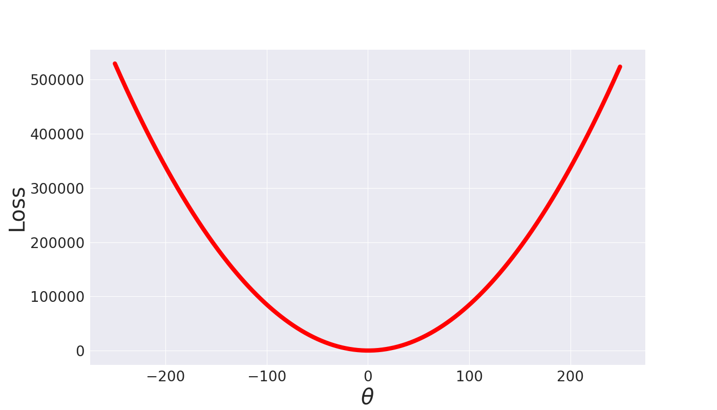
We use \(\hat{\theta}\) as the empirical estimate of the \(\theta\). \(\eta\) is the learning rate and \(\nabla L\) is the gradient of the loss function with respect to \(\theta\). We can write \(\nabla L = \frac{\partial L}{\partial \hat{\theta}}\). One can think of why the gradient descent works. If the loss function is convex means it has “U” shape as shown in the figure below, the “gradient” of the loss function at a point is the “direction and rate of fastest increase”. But we want to minimize the loss, so the idea is to take repeated steps in the opposite direction of the gradient. Opposite direction leads to the fastest decrease of the loss function. You can play with the loss function as a function of \(\theta\) in this python code .

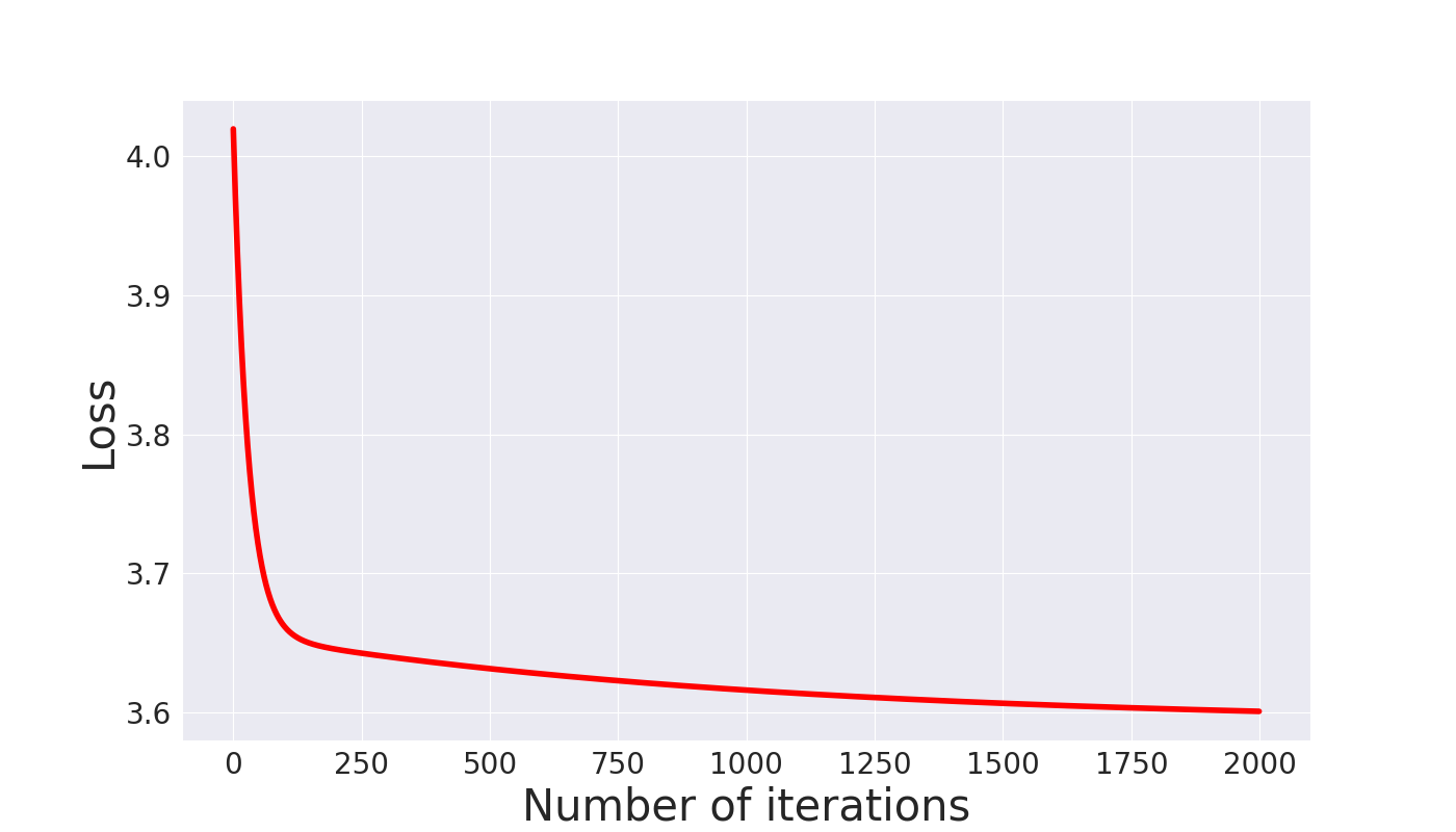
The magnitude of the learning rate \(\eta\) decides the size of the step in the optimization/learning process.

As can be seen in the figure below the loss decreases as the number of iterations increase as we discuss before. Please change the learning rate and the number of iterations in the attached python code and see the behaviour of the loss as a function of iterations and learning rate. There are a few figures inside attached code.

We show the lines that fit the data points for all the three methods(approximate solution using sklearn, approximate solution from scratch, and exact solution). The figures are given below:

Ridge Regression

Here, we try to solve a problem of the form as follows:

\[min_{\theta} ||X\theta - Y||_2^2 + \lambda ||W||_2^2\]

In the above equation , the additional term is known as the regularization loss. \(\lambda\) is the regularization hyperparameter that controls the trade-off between the actual loss and regularization loss. One obvious question can be on someone’s mond why do we add the extra term in the loss function. We can solve this problem in two ways:

Exact Solution

The loss for the \(n\) data points is as follows:

\[L = ||X\theta - Y||_2^2 + ||\theta||_2^2\]

We need to find \(\theta\) that minimizes the \(L\) term.

\[ \begin{align}\begin{aligned}L &= (X \theta - Y)^T(X \theta - Y) + \theta^T \theta\\ &=(\theta^T X^T - Y^T)(X \theta - Y) + \theta^T \theta\\ &= \theta^T X^T X \theta - \theta^T X^T Y - Y^T X \theta + Y^T Y + \theta^T \theta\\ &= \theta^T X^T X \theta - 2 Y^T X \theta + Y^T Y + \theta^T \Theta\\\frac{\partial L}{\partial \theta} &= 2 \theta^T X^T X - 2 Y^T X + 2 \theta^T\\ &= 0\\\theta^T X^T X - \theta^T &= Y^T X\\X^T X \theta - I \theta &= X^T Y\\(X^T X - I) \theta &= X^T Y\\\theta &= (X^T X - I)^{-1}X^T Y\end{aligned}\end{align} \]

Where \(I\) is an identity matrix of \(d \times d\).

Now we have \(\theta\), we can estimate the new output \(\hat{y}_{n+1} = x_{n+1} \theta\). There are some drawbacks in the exact solution:

1. If \(n\) is very large, it is computationally very expensive to process all \(n\) points together. Specifically, the time complexity to find an inverse of an matrix is \(O(n^{2.373})\).

Approximate Solution

Lasso Regression

Baysian Ridge Regression

Click on my

Random Forest Regression

Please see the code .. image:: images/jupyter_python.png

width:

50 px

align:

right

target:

https://colab.research.google.com/drive/1BI1GGxJKHtnADoZvYhRYMcfanZ3NdXlK?usp=sharing

Please try the code.